
Lumen Pro 2 Documentation
Blender lighting addon — your pro tool for handling and analysing illumination data. User manual.
Chapters
1. Introduction to the Blender Lighting Addon
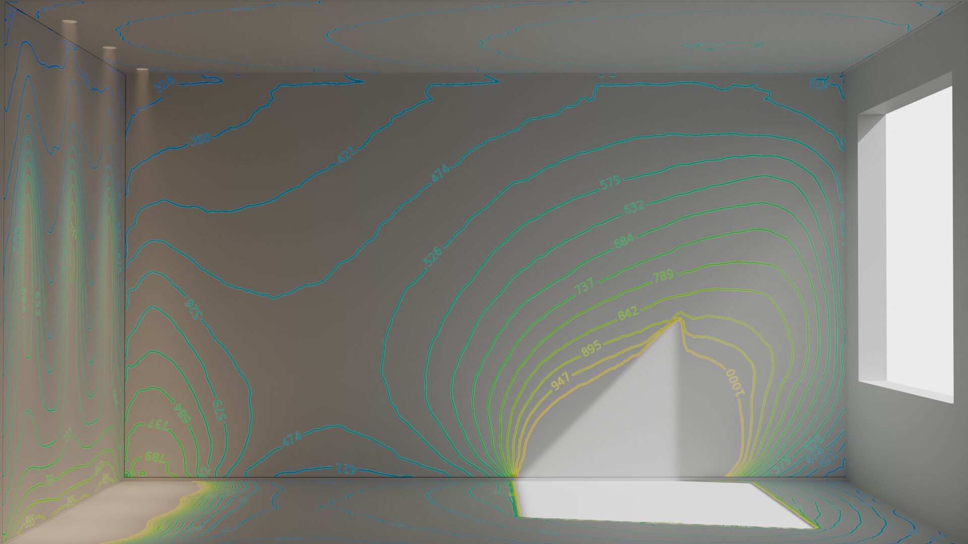
Your Pro Tool for handling and analysing Illumination data.
Lumen Pro 2 is a Blender lighting addon for lighting designers, engineers and visualization specialists. It turns Blender & Cycles into a daylight and electric-light analysis environment: import real photometric data (IES / LDT / GLDF), build physically accurate lighting scenes, calculate and visualize illuminance, and export reports — all inside Blender.
What Lumen Pro can do
- Photometric lights: Import IES and LDT light profiles, or convert existing Blender lights, and get a real Cycles light that emits exactly according to its candela distribution.
- GLDF / L3D: Import the lighting-industry GLDF product format with geometry, joints, emitters and photometry.
- IES library: Browse a folder of IES/LDT files with thumbnail previews and apply or convert profiles in one click.
- Analysis planes (Lumen Graph): Bake illuminance to any flat mesh, get DIN EN 17037-style statistics and visualize results as textures, bars, values or matplotlib ISO lines.
- Realtime tools: Interactive probe, calculation and iso-contour overlay modes with live viewport feedback and uniformity ratios.
- CIE sky & weather: Physically based CIE standard skies, EPW weather data, accumulated skies and custom sky imports for daylight studies.
- Glazing: Import angle-dependent window optical data (e.g. from LBNL’s WINDOW program) into realistic window materials.
- Compositor legend: Generate color legends for your analysis images right in the compositor.
- Export: A4 matplotlib reports, ISO-line overlays from your render, and per-pixel CSV data of any analysis plane.
Requirements
| Software | Blender 5.1 or newer |
| Render engine | Cycles — required for importing lights, baking and most features |
| Platforms | Windows x64, macOS (ARM), Linux x64 |
| License | A Lumen Pro license key is required to activate the add-on (see chapter 2). |
2. Installation & License
System requirements
| Blender | 5.1 or newer |
| Platforms | Windows x64, macOS (Apple Silicon), Linux x64 |
| Python | 3.13 (bundled with the supported Blender versions) |
| Render engine | Cycles — required for importing lights, baking and most features |
Installation (Extension Repository)
Lumen Pro 2 is distributed as a Blender extension through the Lumen Pro extension repository. The quickest way is to drag and drop the button for your operating system into the Blender window — Blender adds the Lumen Pro repository and offers the add-on for installation:
- First drop — adds the Lumen Pro repository to Blender and offers the add-on for installation.
- Second drop — installs the add-on if it was not offered right after the first drop (or instead: open Edit → Preferences → Get Extensions, press Install and then Enable; use Refresh Remote in the Repositories tab if it does not show up).
While the add-on is being downloaded / installed Blender’s interface locks briefly — this is normal, just wait until it finishes. Do not force-quit Blender during the install.
Manual installation (step-by-step) — if the drag & drop did not work
Install it manually:
- Open Blender and go to Edit → Preferences → Get Extensions.
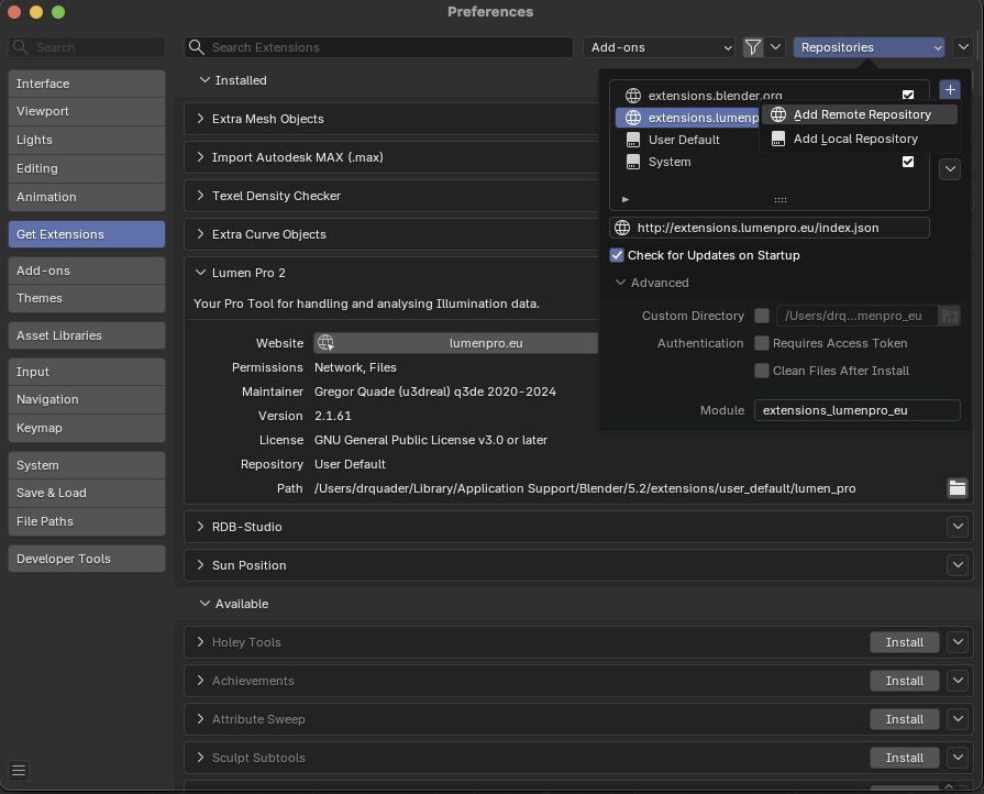 Figure 2-1 — Open Preferences and switch to Get Extensions.
 - Open the Repositories tab (or the repository dropdown) and add a new remote repository with the little arrow / + button.
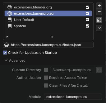 Figure 2-2 — Repositories → the + / Add Remote Repository.
 - Set the repository URL to
https://extensions.lumenpro.eu/index.jsonand confirm. - Refresh the repository. The Lumen Pro 2 add-on will appear in the list.
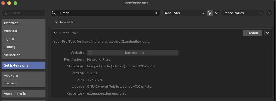 Figure 2-3 — Lumen Pro 2 is now listed under Available Extensions — press Install.
 - Click Install and then Enable Lumen Pro 2. Use the little arrow on the right to open View Details.
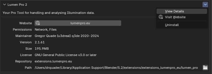 Figure 2-4 — The little arrow on the right opens View Details / the add-on preferences.
 - Tip: enable automatic updates for the repository to always get the latest version.
https://extensions.lumenpro.eu/index.json.
A wrong URL gives no error message, the repository simply stays empty.
Activating your license
Lumen Pro is a paid add-on. After purchasing you receive a license key by e-mail. To activate the add-on:
- Go to Edit → Preferences → Add-ons and find Lumen Pro 2.
- Open the add-on’s preferences section (Lumen Pro LIC Key).
- Paste your license key into the Lumen Pro LIC Key field and press Enter.
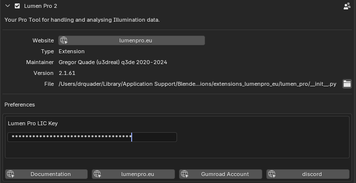 Figure 2-5 — Paste your license key into the Lumen Pro LIC Key field and press Enter.
 - The key is validated immediately. When activation succeeds your UUID is shown and the status message confirms the license.
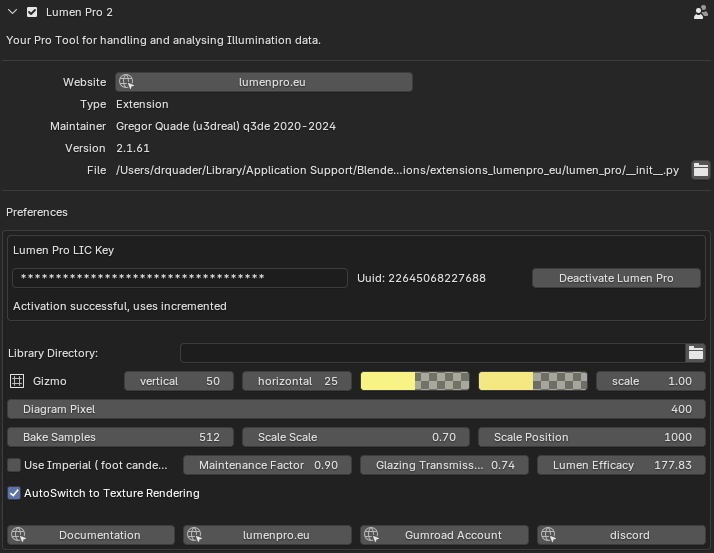 Figure 2-6 — Activation succeeded: the license is valid and the add-on is fully functional.
 - Once active, the add-on is fully functional. The full set of preferences is described in chapter 14.
Deactivating a license
Each license key can be activated on a limited number of machines. If you switch computers or give a machine away:
- Open Edit → Preferences → Add-ons → Lumen Pro 2.
- In the preferences section click Deactivate Lumen Pro first.
- Afterwards the key can be activated again on another machine.
You can also manage your activations online in the Lumen license admin panel — log in with your email and license key to view and deactivate machines from anywhere.
3. Quick Start
The goal of this chapter: get a real photometric light into your scene and run a first illuminance analysis — in a few minutes.
- Open Blender and select Cycles as render engine (render properties → Render Engine). Lumen Pro lights, baking and most tools require Cycles.
- Make sure the add-on is activated and the license is active (see chapter 2). Blender should have internet access for the license check.
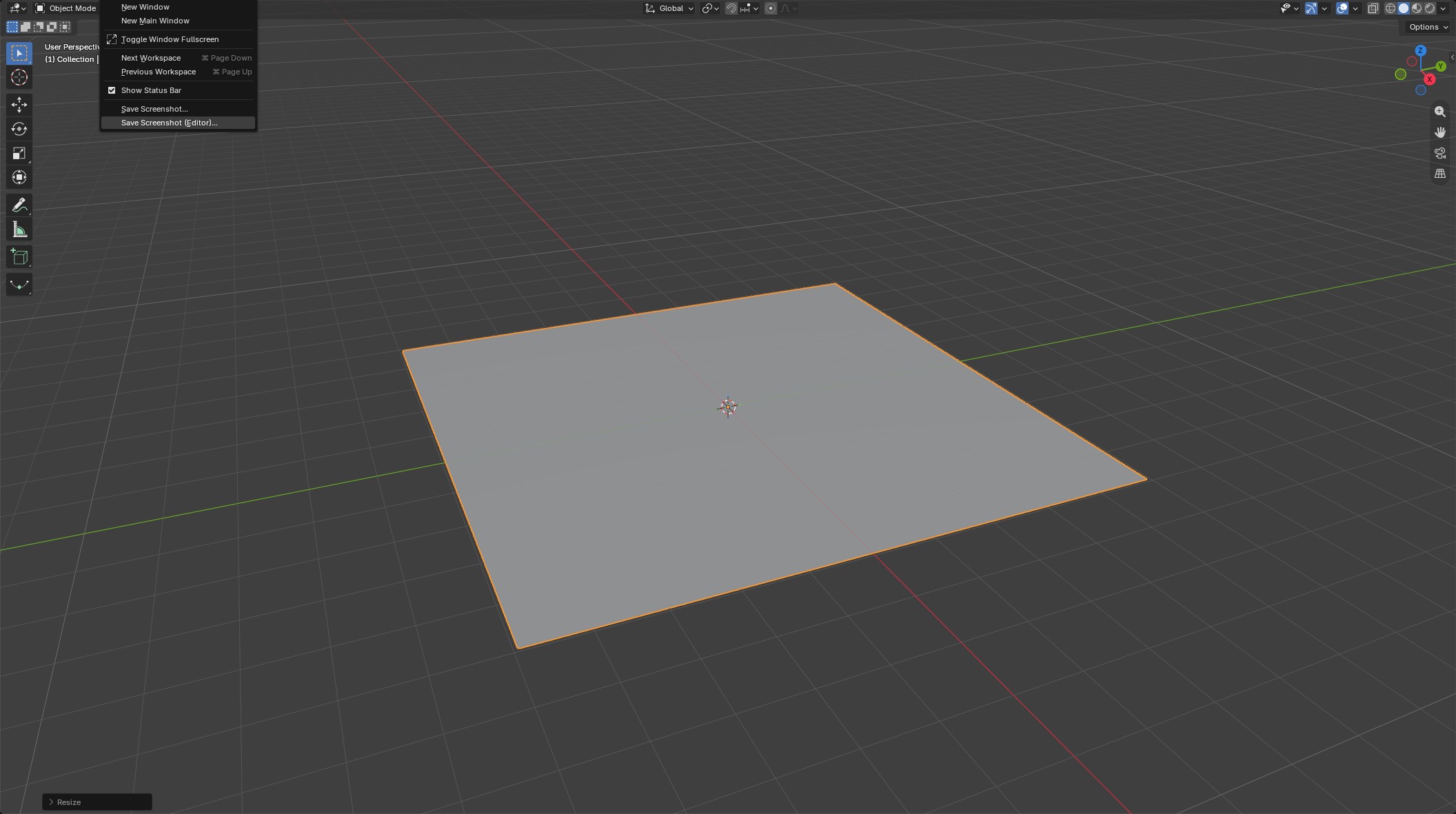
- Set up a simple scene you can analyze: e.g. add a Plane (Shift+A → Mesh → Plane) for the room floor, and optionally a box for a room.
Step 1 — Add a photometric light
There are two ways to add an IES / LDT based light:
- Add menu: Shift+A → Light → Photometric (or GLDF / L3D for GLDF files).
- Lumen Pro tab: in the 3D Viewport open the N-panel (press N), switch to the Lumen Pro tab, and in the Import box click IES / LDT.
Select your .ies, .ldt or .LDT file. The operator asks for a Color Temperature (e.g. 4000K) and a name. Lumen Pro builds a Cycles light that emits exactly according to the file’s candela distribution.
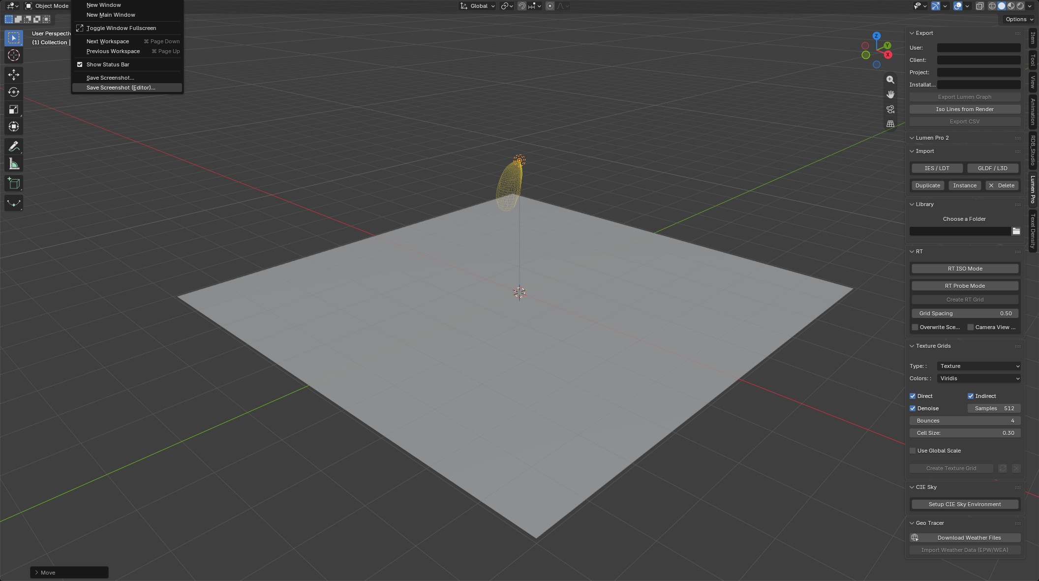
.ies / .ldt file.Step 2 — Place and aim the light
The light is added at the 3D cursor. Move and rotate it like any Blender light. In the viewport you see an IES mesh gizmo previewing the photometric distribution — it updates live while you move, rotate or scale the light. Scale the light object to change the luminous size.
Step 3 — Inspect the light data
Select the light and switch to the Light properties (lightbulb icon). The Lumen Pro panel shows:
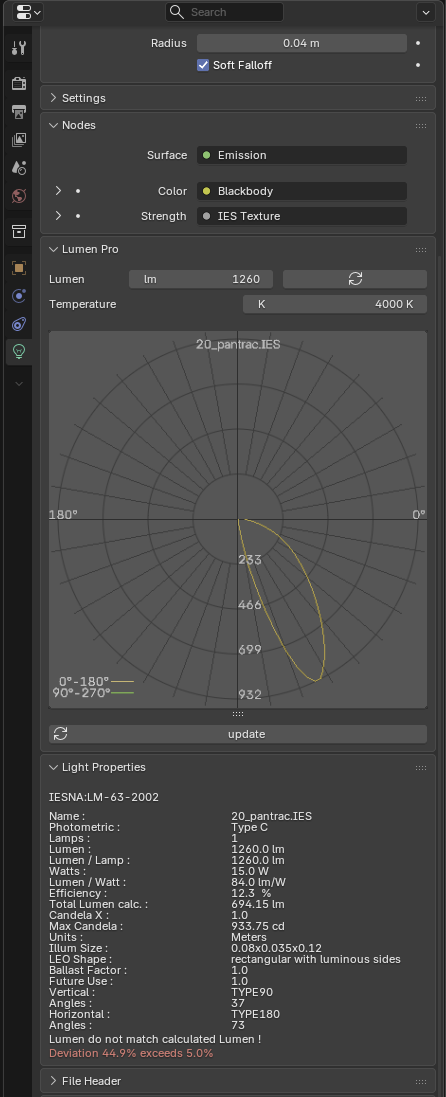
- lumens, temperature (Blackbody, editable in Kelvin),
- IES data summary — name, photometric type, lamps, total lumens, candela values, watts, efficacy,
- a preview of the polar diagram / profile.
Step 4 — Run a first analysis
- Select a flat mesh that will be the analysis surface (e.g. the floor plane).
- Press L and choose Create Lumen Graph — Lumen Pro converts the mesh into a texture grid and bakes the illuminance automatically.
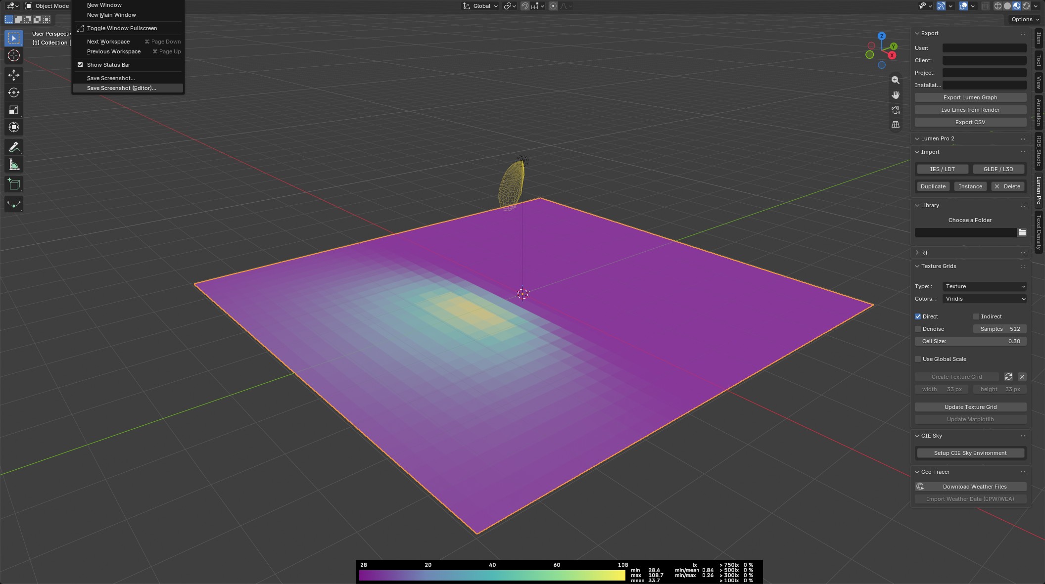
ISO lines, curves and the realtime (RT) modes are covered in their own chapters later in this manual.
4. Photometric Lights
A photometric light is a Cycles light that emits exactly according to a real luminaire’s candela distribution, defined in an IES or LDT photometric file. Lumen Pro reads the file and builds a node setup with an IES texture, a blackbody temperature and its luminaire group (Lumen_point or Lumen_area).
Creating a new photometric light
- Make sure Cycles is the active render engine (Lumen Pro refuses to import otherwise).
- Add the light: Shift+A → Light → Photometric, or open the N-panel (Lumen Pro tab) and click Import → IES / LDT.
- Pick your file (as well as listing
.iesand.ldt, the loader also accepts the uppercase.LDTextension common on Windows). - Choose a Color Temperature (1700–20000K) and, if you like, a Name. LDT files are converted to IES internally.
- Confirm. A point light is created at the 3D cursor with the full Lumen node tree wired up.
The toggle Use Area Light in the Lumen Pro N-panel (Library section) switches the import to an area light instead of a point light.
Converting an existing light
You can also turn an existing Blender light into a photometric one:
- Select the light object(s) you want to convert.
- Run Import → IES / LDT in the N-panel and pick the photometric file (or use Convert from the library).
- Confirm the color temperature. The light keeps its location and scene placement, while its data and node setup are replaced by the IES-based network.
The light data panel
Select a photometric light and switch to Light properties (lightbulb icon). The Lumen Pro panel shows:
- Lumen — editable total luminous flux in lm with a reset button (returns to the file’s value).
- Temperature — the blackbody temperature in Kelvin (also editable in the node editor).
- A live preview of the photometric profile, plus a summary table with all file data — name, IESNA format version, photometric type, number of lamps, total / per-lamp lumens, watts, lm/W, efficiency, maximum candela, dimensions, LEO shape, ballast factor, lamp mounting type and the vertical / horizontal angle counts.
Maintenance factor
Every Lumen light applies the Maintenance Factor preference (default 0.9) through its node group. Changing the preference updates all existing Lumen lights automatically.
lumen_type property.
A full description of the IES profile file is available in the node setup; the polar diagram gizmo is covered in
chapter 7 and chapter 8.
5. GLDF / L3D
GLDF (Global Lighting Data Format) is an open XML/ZIP container for complete luminaires.
It bundles the 3D geometry (L3D) with the photometric measurements, light-emitting
objects / surfaces, and product information. Lumen Pro imports the file through
File → Import → GLDF / L3D (*.gldf, *.l3d),
or via the N-panel Import → GLDF / L3D. Cycles must be the active render engine.
Importing a GLDF product
- Run File → Import → GLDF / L3D (or the N-panel import button) and pick a
.gldffile. - A preview dialog opens with the product Name and Description read from
product.xml. - Choose one of the available Variants (each variant groups a specific emitter + geometry combination of the product).
- Click Import. Lumen Pro imports the L3D geometry with joints and positions,
attaches an empty with
lumen_type = 'GLDF'as the luminaire origin, imports the OBJ geometry with its materials and textures (units converted: cm/mm → m), and parents the photometric lights to the luminaire objects so the whole assembly moves as one.
If you pick a file whose data contains no product.xml or no valid
variant, the import is cancelled and an error dialog is shown.
Joints
L3D files can define adjustable joints (e.g. for pendants and gimbal rings).
Lumen Pro reconstructs the joint hierarchy: each joint is an empty at its declared position and
rotation, sized to the part, and the child geometry is parented to it. Joint rotation limits from the
L3D file become Limit Rotation constraints. Select the luminaire origin empty
(a GLDF object) and open the GLDF tab in the 3D Viewport N-panel
(GLDF Joints panel): it lists every joint and provides editable
X / Y / Z rotation fields in degrees, each showing its allowed range
(e.g. [-15.0° ... +15.0°]) so you can aim the light within
its mechanical range.
Light-emitting objects & surfaces
- Luminaire objects (LEO) and luminous surfaces (LES) from the L3D structure are represented in the scene, matching the real emitting parts of the fixture.
- The photometric data of the GLDF variant (“ldt” file) is applied to the emitted light as a Lumen Pro photometric light (IES/Polar grid) parented to the object. The Use Area Light toggle again selects a point or area emitting surface.
Tips
- The luminaire origin empty (visible as plain axes at the product mount point) is the convenient handle for placing and rotating the entire product.
- Photometric data and all Lumen Pro node groups behave exactly like the lights described in chapter 4 — edit lumens, temperature and inspect the data panel afterwards.
- Use the L-pie menu “Update Lumen Graph” after moving geometry if you already baked analysis for the imported scene.
6. IES Library
The IES library turns a folder of photometric files on your disk into a visual, thumbnail-based browser. You can browse IES / LDT files with a real preview render of their luminous distribution and add, convert or apply a profile in a single click — without touching the file picker for every single light.
Preparing the library
- Open Edit → Preferences → Add-ons → Lumen Pro 2.
- Set Library Directory to the global folder that stores your IES profiles (the folder is scanned for
.ies,.IES,.ldtand.LDTfiles).
Browsing the library
- In the 3D Viewport open the N-panel (Lumen Pro tab) and expand the Library box. If the folder is empty you’ll see “Choose a Folder” and can point the browser at another directory.
- The first time you open it, Lumen Pro renders a preview thumbnail of every file in the folder (a small Cycles render of the IES profile) and stores it in a
previewssubfolder. Depending on the folder size this can take a moment. - Use the refresh button (
FILE_REFRESH) to re-render previews, e.g. after you added new files to the folder. - If the folder has subfolders, a subfolder dropdown appears above the grid — pick one to browse it (the
previewsfolder itself is skipped). - The grid shows the thumbnails; hovering shows the parsed file description (manufacturer, lumen, watts, catalog …). Click a thumbnail to select it — the filename is shown below the grid.
Add, Convert or Apply
With a profile selected, the Library box offers three actions, depending on your selection:
| Add | Creates a new photometric light at the 3D cursor with the selected profile, named after the file. Like chapter 4 imports — Cycles must be active. |
| Convert | Turns the selected existing Blender light(s) into Lumen Pro lights with the selected profile, keeping their location and name. |
| Apply | Swaps the photometric file of the active Lumen Pro light to the currently previewed profile — a lightweight update that keeps the existing node setup (shown instead of Convert when the light’s profile differs from the previewed one). |
The Use Area Light toggle (below the grid) maps the profile onto an area / luminous surface instead of a point light.
A note on physics: photometric data is captured in spherical format, so mapping it onto a flat area light is an approximation rather than physically exact. The results are nonetheless very close, because Lumen Pro maps the total luminous flux (energy) over the whole emitting area — which makes rendering noticeably more realistic (soft shadows, luminous size of the fixture). The trade-off: for rendered light this behaviour is limited to 90° vertical profiles (Type 90). For vertical Type 180 files an area light is not suitable — Lumen Pro then shows a warning popup (“Area Lights are not suitable for vertical TYPE180 ! May alter Illumination !”) — use a point light for those. Also note that the luminous panel itself only appears in the final render / camera view when its camera visibility is enabled — if the light does not show up on camera, enable its camera visibility in the light’s ray visibility settings.
The L key “Lumen Pro” pie menu
Press L in the 3D Viewport:
- Add from Library — same as the “Add” button, using the currently selected thumbnail.
- Apply from Library — appears when a Lumen Pro light is active whose profile differs from the previewed file.
7. Analysis Planes (Lumen Graph)
A Lumen Graph (also called lightplane / texture grid) is a flat mesh that Lumen Pro converts into an illuminance analysis plane: it bakes the incident light onto an image texture, computes DIN EN 17037-style statistics and visualizes the result on the mesh — as textured values, 3D bars, numeric geometry or matplotlib ISO lines.
Creating an analysis plane
- Select a flat mesh that will be the analysis surface (the floor of a room, a work plane …).
The object must not be a Lumen object yet (no
lumen_type). - Create the plane: press L → Create Lumen Graph, or use the Create Texture Grid button (N-panel → Lumen Pro → Texture Grids).
- The object is renamed Lumen_Graph and tagged
GRAPH. It is excluded from light transport (no rays bounce off it), receives the Lumen_data_vis material with its baked-image node, and the texture resolution is derived from the graph’s footprint and the cell size: resolution = plane width / cell size per axis.
Creating a graph bakes it immediately — you get the illuminance result right away. The bake runs Cycles with the samples from the Bake Samples preference (default 512) and converts the render to lux using the lumen efficacy preference.
Texture Grid from Faces (click-to-graph)
Instead of converting an existing mesh to a graph, you can click faces of a larger mesh (a building floor, a room, …) to create one or more analysis planes directly on the surface. The source mesh is never modified — each graph is a separate new object.
- Select a mesh (e.g. a room floor). Press L → Texture Grid from Faces, or use the button in the N-panel → Lumen Pro → Texture Grids → boxed section.
- Hover a face — it glows yellow. Click to select (turns orange). Hold Left Mouse and swipe to paint-select multiple faces.
- Press N to commit the current selection as a separate grid group (committed groups are shown in teal). You can now select faces for the next grid.
- Press Right Mouse or Enter — every committed group (plus any remaining selection) becomes its own Lumen_Graph grid, baked and ready, and the modal exits.
- Esc — cancel and exit without baking.
In the N-panel box you can set:
- Fast Shot — each click immediately creates and bakes a single-face grid (no selection mode).
- Offset — work-plane height above the surface (default 0.001 m to avoid z-fighting).
- Hover Filter — controls which faces can be hovered / selected:
- Front-Facing (default) — only faces whose front side faces the camera. Viewing from above this naturally selects only floors, skipping ceilings and walls seen edge-on.
- Floors — only faces that face upward (world +Z).
- All Faces — no filtering (original behaviour).
Display types
In the N-panel Texture Grids section, Type chooses how the result is drawn:
| Texture (default) | Shows the baked illuminance image mapped on the plane. |
| Mathplotlib | Overlays matplotlib ISO lines / filled contours / grid numbers on the plane. Configure via Colors, Style, Line Width, Levels, Font Size, Grid Size, Mathplot Multiplier. |
| GEONodes–Bars | Builds true 3D bar geometry from the texture via a Geometry Nodes modifier (Lumen_bars). |
| GEONodes–Values | Builds numeric value geometry showing the lumen values on the plane (Lumen_Values). |
After switching the type, run Update Texture Grid (or the L-key Update Lumen Graph) to rebuild the display. Update Matplotlib refreshes only the ISO lines without re-baking.
Statistics & DIN EN 17037
Every bake computes, from the valid pixels of the analysis plane:
- min / max / mean illuminance,
- uniformity ratios min/mean and min/max,
- the percentage of the plane above 100 / 300 / 500 / 750 lx — the building blocks of DIN EN 17037 daylighting assessments.
The bake resolution is controlled by Cell Size — the smaller the cell, the higher the texture resolution (texture width / height = plane size ÷ cell size per axis). The panel shows the resulting Texture size (W × H px) as a read-only readout. The default Graph Cell Size is 0.3 m, which matches the cell size used in the DIN EN 17037 example. To change the resolution later, edit Cell Size and run Update Texture Grid — the texture is re-sized and re-baked automatically, no reset or re-create needed. The values are shown as an on-screen legend / scale bar with the 5-step color ramp once the graph is selected. Global Scale lets you fix a shared min/max range across several graphs so their colors can be compared directly.
Update and clear
- Update Texture Grid — re-applies the current Cell Size (re-sizing the texture if needed) and re-bakes after you move light-fixtures, geometry or change the cell size.
- Update Matplotlib — re-renders ISO lines from the existing bake at the resolution set by the Mathplot Multiplier.
- Clear Lightplane — removes the graph behaviour, statistics and material (back to a plain mesh).
8. Realtime Tools
The realtime (“RT”) tools compute illuminance live in the viewport while you work. They only act on Cycles Rendered shading — activating a mode switches the viewport to Rendered and snaps cursor placement to faces. Everything is local and does not change your scene data (probes are empties you can delete anytime).
RT Probe mode
- Activate Rendered shading (or press L and toggle Lumen RT Mode in the pie menu).
- Hold Ctrl+Alt and release the left mouse button on the surface you want to measure — a probe empty (Lumen_RT_Probe) is placed exactly at the clicked point on the surface, with its arrow oriented along the face normal (so the value label floats above the surface, following its slope).
- Each frame Lumen Pro samples one pixel under the probe and displays the value next to it, plus min / max / mean and uniformity edges on the whole line of probes.
- While RT mode is active you can also grab a probe (G) and hold Ctrl to snap it onto another face — it is placed on the surface and its arrow automatically aligns to that face’s normal, so the value label keeps floating above the surface, following its slope.
- Set the displayed unit in the N-panel RT box: W/m² (irradiance), Lux, cd/m² (luminance), Footcandles or Daylight Factor (%).
- Adjust Font Size, Min Size (empty height floor) and Size Multi (height scaling of probes) while Hide Label / Show Label toggles the numeric readout.
- Save the view with Save RT Screenshot (N-panel → RT box at the bottom, or the L-pie menu): it opens a file browser and saves the current 3D viewport — probes, value labels and rendered scene — as a PNG.
- Exit with ESC (or toggle Exit RT Mode in the pie menu).
RT Grid
- Select a flat mesh and press L → Create Lumen RT Grid (or the Create RT Grid button in the RT box).
- The mesh is renamed Lumen_RT_Graph (
RT_GRAPH) and a probe empty is created on every grid point. The Grid Spacing value (default 0.5 m) controls the probe density. - Activate Lumen RT Mode afterwards — the whole grid now shows live values and statistics.
RT ISO mode
- Press L → Lumen RT ISO Mode (or the N-panel toggle). The viewport runs the live contour shader over the rendered scene.
- Configure in the N-panel RT box: Line Width, Line Alpha, Line Levels, Min / Max lux, Use Bands (filled contour bands instead of lines) and Colors (matplotlib colormap).
- With Camera View Only the analysis is limited to the camera view frame; without it the whole viewport is covered.
- Overwrite Scene Materials replaces materials with a neutral Lumen_overwrite material during the mode, so the ISO colors are easier to read — the original materials are restored on exit.
- A color scale bar and min / max / mean stats are drawn on screen.
- Save RT Screenshot (N-panel → RT box at the bottom, or the L-pie menu) captures the current viewport with the ISO overlay as a PNG via the file browser — handy for sharing contour results without a full render.
ISO from a render
The Iso Lines from Render button (N-panel → Lumen Pro → Export) renders the beauty frames through the same contour shader offline and stores the result as the packed image Lumen_ISO_Overlay. The image can be used in the compositor to overlay the iso lines onto your render for the final output — see chapter 9.
A camera and a rendered render result are required: make sure the scene has a camera that frames your analysis, render the image first (image → any frame of the animation), and then run Iso Lines from Render. It reads the last render result present in Blender, so there is nothing to overlay without a rendered image.
9. Compositor tools
Lumen Pro ships a set of premade compositing node groups and a legend generator. The node groups let you build flexible overlays — for example the same look as the realtime ISO lines (chapter 8) — but composited through the node editor: you can regenerate, recolor and recombine them live, on top of any render or viewport stream.
Enabling compositing (Blender 5.1 and newer)
Lumen Pro supports Blender 5.1 and up, where the old “Use Nodes” toggle no longer exists. Compositing is driven by a compositing node group attached to the scene:
- Open a Compositor editor (switch an editor type to Compositor).
- In the Compositor header, click New to create a compositing node group. It becomes active for the current scene and is used by the render pipeline and by the realtime compositor.
- Enable the Realtime Compositor in the 3D viewport header (the realtime-compositor dropdown → Realtime or Always) so the composite shows live in the viewport while you work — switch it off for full-performance viewport previews.
- Make sure a Group Output node is present; if it is missing the compositor does not run.
Premade node-group assets
Lumen Pro registers its assets folder as the Lumen Pro asset library, which includes the
pre-built compositor_nodes compositing node groups. Append a group from the asset
browser (or from File → Append) inside your compositing group — several can be wired together:
- lumen compose — the base group: Render Layers → Exposure → Group Output. Use it as the backbone of your compositing setup.
- Analysis overlays —
colorramp min max,Daylight Factor,DayLightFactor,area greater thanandarea less thanrecolor image regions by value, e.g. to highlight the iso-contour look from chapter 8. - Line styles —
line,single_line,three linesanddotsdraw contour-style line/hatch overlays over the image. - Unit conversion —
Units,W/m² to lux,W/m² to fcandrgb to W/m²convert between irradiance, illuminance and raw image values. - Place Legend — places a legend image onto the frame (used together with the legend generator below).
The legend tool
The legend generator is one of the compositor tools: it creates a color legend image for your analysis and inserts it into the compositing node group, so an annotated scale is composited into the final frames. Its Lumen Pro Legend panel appears in the N-panel of the Compositor editor.
Legend items list
- Click Add Legend Item to add steps. Each item has a value (a lux level), a color and a style (area bar or thin line). Use the + / − / up / down buttons to manage the list; values of new items step by 100 lx and cycle through rainbow hues as defaults.
Layout
- Width (default 200) and Height (default 400) of the legend image.
- Margin (default 20) around the contents.
- Label (e.g. “Illuminance”) and Unit (e.g. “lx”) become the header Illuminance [lx] on top of the legend.
- Font Color and Background Color for the legend.
- Image Name — the Blender image that receives the legend (default
Lumen_Legend).
Generating
- Click Generate Legend Image. Lumen Pro renders the legend offscreen (GPU), packs it into the named image and inserts an Image node with it into the compositing node group at a convenient position.
- Connect the node’s Output into your setup (e.g. combined via
Place Legend, a Mix, or an Overlay) so the legend lands where you want it in the frame — in Blender 5.1+ results flow to the Group Output node. - With the realtime compositor enabled, the legend appears live in the viewport; render to bake it into the frames.
10. CIE Sky & Weather Data
Lumen Pro generates physically based CIE standard skies and combines them with real EPW climate data for daylighting analysis. The sky is baked into an equirectangular High-Dynamic-Range environment image and plugged into the World background of your scene.
Setting up the sky
- Open the N-panel → Lumen Pro tab → CIE Sky box.
- Click Setup CIE Sky Environment. Lumen Pro builds the world shader (Lumen_CIE_Sky_Env environment texture → Background → World Output) and generates the initial sky image.
- Pick a Sky Type — from the CIE standard series (overcast 1–5, partly cloudy 6–11, clear skies 12–16) plus the Perez all-weather model (default).
- Set the daylight via Sun Altitude, Sun Azimuth, DHI (diffuse horizontal irradiance) and DNI (direct normal irradiance). If Include Sun is on, a bright solar disc is baked directly into the texture — there is no separate sun light object, which keeps the analysis clean.
- Ground Reflection controls the ground luminance (DHI/π · reflection).
- Choose a Resolution (Low 256×128 up to Ultra 2048×1024, or Custom) and click Update Sky Texture. Enable Auto Update to regenerate automatically whenever a parameter changes.
EPW weather data
EPW files (EnergyPlus / Ladybug) provide per-hour climate data for any location:
- Click Load EPW Data and choose a
.epwfile. Lumen Pro reads the location (latitude / longitude / timezone from the header) and the hourly GHI / DNI / DHI (plus their illuminance equivalents and zenith luminance). - The Ev,d,med value (the median daylight illuminance of the brightest half of the year) is computed automatically — this is the reference value used for daylight-factor-based assessments.
- The EPW fields now drive the Month / Day / Hour (and day-of-year) sliders: choosing a date & time sets the sun position and irradiances from the weather file, so the sky matches the real sun ” for that moment.
Accumulated sky
With EPW data loaded you can aggregate many sky states into one average sky:
- Enable Calculate Accumulated Sky in the Accumulated Sky box.
- Set the start / end date (month, day, hour) and the Time Step in hours (minimum 1 minute).
- Click Calculate Accumulated Sky. Lumen Pro walks the EPW data through the range, computes a CIE sky for each step and sums them into one image (Lumen_Accumulated_Sky) that is plugged into the world — your annual average daylight situation as a single environment.
The calculation runs in the background: Blender stays fully responsive while a progress bar in the viewport shows the percentage and step count. Press ESC to cancel at any point. The Chunk Size (steps processed per frame, adjustable in the F6 redo popup before starting) trades calculation speed against UI responsiveness — larger chunks finish faster but make Blender less responsive.
Import CIE Sky (CSV)
The Import CIE Sky button loads a per-patch sky CSV (Tregenza-style subdivision with direct beam / diffuse horizontal data) and rasterizes it into the same equirectangular environment, useful for external sky-model / simulation tools.
Geo Tracer & realtime CIE skies
For realtime sky analysis in the viewport, Lumen Pro provides the Geo Tracer workflow: a Geometry Nodes based tracer that evaluates the CIE sky (and EPW weather) inside Blender’s node graph. See the next chapter.
11. Geo Tracer (Realtime CIE Sky)
Geo Tracer is Lumen Pro’s Geometry-Nodes based tracer for realtime daylight analysis. Instead of baking a static environment image, it evaluates the CIE sky and weather data directly inside Blender’s node graph — so moving the sun, changing the date or the sky model updates the illumination live in the viewport.
It ships as custom geometry node groups (Lumen Sun Sky, Lumen Accumulative Sky) that you add to your analysis mesh from the asset library. The whole sky / weather model lives in the node tree and can be combined freely with other geometry nodes.
Geo Tracer panel
The N-panel → Lumen Pro tab → Geo Tracer box provides weather data tools for the node groups:
- Download Weather Files — opens the EPW weather map (ladybug.tools / EPWmap) in your browser so you can fetch real climate files for your location.
- Import Weather Data (EPW/WEA) — loads an
.epwor Radiance.weafile. The operator writes two CSV files next to your weather file (weather_data.csvwithmonth, day, hour, dni, dhirows, andweather_meta.csvwithlat, lon, tz, elevation) and wires them into the CSV sockets of the node group on your active Lumen mesh — the tracer can then drive the sun position and irradiances from the real hourly data.
Workflow
- Create or select the analysis mesh you want to shade with the tracer.
- Add a Lumen Sun Sky node group (from the Lumen asset library) as a Geometry Nodes modifier. The operator requires a Lumen object with a node-group modifier to import weather data.
- (Optional) Import your EPW / WEA weather file from the Geo Tracer panel — it fills the node’s weather_csv / meta_csv sockets with the generated CSVs.
- Drive the node inputs for date, time and sky type. The viewport reflects the daylight conditions in realtime.
Node groups
All Geo Tracer node groups are part of the Lumen Pro asset library
(geo_nodes) and are evaluated by Blender normally. The two main tracers:
- Lumen Sun Sky — the realtime tracer. Inputs: name, weather_csv / meta_csv, the month / day / hour start+end range, and the display toggles Compass, Analemma, Sun Vectors and Limits.
- Lumen Accumulative Sky — aggregates many sky states into one result. Adds the Subdivision Type and Sky Components menus and the Accumulate in Sensor toggle; it sums hourly contributions over the selected date/hour range (for annual / seasonal averages on a sensor grid).
- Lumen CIE Sky — a single, static sky state from Day Of Year, Sun Altitude / Sun Azimuth, DNI / DHI and Dew Point — useful when you do not need weather data.
Supporting groups round out the tracer: Lumen Compass, Lumen Date, Lumen Location, Lumen Day Of Year, the sensor grid (Lumen Sensor, Lumen Sensor Grid / Grid Loop), Lumen Statistics, Lumen Filter EPW Data / Lumen Sample EPW, Lumen Display Values, Lumen Legend, Lumen Texture to Grid and the solar-astronomy / CIE helpers (Sun Vector, altitude / azimuth, decl, eot, ha, lst, tc, the CIE type0 / linear coefficient formula groups and DLA EN DIN 17037 for glare/daylight-assessment shading) — all reusable inside your own geometry-node trees.
12. Glazing
Lumen Pro imports angle-dependent window optics from LBNL’s WINDOW program reports (the de-facto tool for window performance data) into a material, so your daylighting analysis uses the real transmittance / reflectance of the glazing at every incidence angle.
Preparation
- Open the Asset Browser and drag the Lumen Glazing material onto the glazing object. This creates a material whose node tree already contains the required Tvis (visible transmittance), Rfvis (front reflectance) and Rbvis (back reflectance) Float Curve nodes, plus the optional transmittance and reflectance RGB nodes that receive the integrated colors.
- Select the glazing material so it is active (the tool writes into
context.material).
Applying glazing data
- Open the Shader Editor and switch the sidebar (N-panel) to the Node category — the Lumen Glazing panel appears (it shows only for shader/material editing).
- Either pick a glazing from the bundled assets folder (dropdown “Glazing File”) and click
Apply, or load your own report with Import from File (
*.txt). - Lumen Pro parses the WINDOW report (Optical Properties for Glazing System): the incidence-angle table with per-angle Tvis, Rfvis and Rbvis values (the trailing hemispherical average is skipped), and optionally the CIELAB color properties, which are converted to linear RGB and fed into the color nodes.
- The float curves are repopulated with the measured pairs and the material is refreshed. From now on the glass reacts correctly to oblique light, exactly like the measured pane.
13. Export
Lumen Pro provides three ways to get your analysis out of Blender: a formatted illuminance report, a contour overlay image from your final render, and raw per-pixel data as CSV. All of them work on a selected Lumen Graph object and live in the N-panel → Lumen Pro → Export box.
Report header
Before exporting, fill in the User, Client, Project and Installation fields at the top of the Export box. They appear in the report’s left sidebar (Client, Project, Installation, Date, Metric, User) — the date is filled in automatically and the Metric is always Illuminance (lux).
Lights for Export
The Export box holds a Lights for Export list. Use the + button to add the selected light objects to the report, the − button to remove the selected row, and the × button to clear the whole list. Lights added here appear two ways in the report:
- as diamond markers on the graph — one per light, coloured per IES profile and numbered (1, 2, 3 …) in the order of the list;
- as a light profile line at the bottom of the page — a colour swatch plus the profile name, light count, and the representative light’s lumens (lm), candela (cd) and wattage (W).
If the list is empty, the report is exported without any light markers or the bottom light section.
Export Lumen Graph (A4 report)
- Select the analysis plane that holds the illuminance data.
- Click Export Lumen Graph. A file browser opens — pick the Format (PNG or PDF) and the destination file. Lumen Pro saves an A4 landscape report (matplotlib): the logo and report title in the header, the project sidebar (Client / Project / Installation / Date / Metric / User), the results block (Avg / Min / Max in lx, the Min/Avg and Min/Max uniformity ratios, and the % of the plane above 100 / 300 / 500 / 750 lx), and the colour plot of the plane — either the baked ISO-line image or freshly drawn contours following your ISO style, with a colorbar (no label — the Metric in the sidebar covers this) and metered axes (aspect equal). The report resolution follows the Mathplot Multiplier.
Iso Lines from Render
- Select the graph whose range your render represents and click Iso Lines from Render.
- Lumen Pro renders the current frames through the contour shader (see RT ISO), stamps min / max / mean + a mini legend and writes the result into the packed image Lumen_ISO_Overlay in your blend file — ready to combine with the legend of chapter 9.
This requires a camera framing your analysis and a rendered render result present in Blender — render the image first, otherwise there is no beauty frame to draw the contours onto.
Export CSV
Raw data export for further processing (e.g. in Excel / CAE tools):
- Select the graph and click Export CSV.
- Choose a destination file. For every pixel of the analysis plane the CSV writes one row with: X / Y / Z world coordinates (m), the pixel area (m²), the visible irradiance (W/m²) and the illuminance (lux).
14. Preferences Reference
All add-on settings live in Edit → Preferences → Add-ons → Lumen Pro 2. They are split into sections; most appear only while the license is active.
License
| Lumen Pro LIC Key | Your license key (see chapter 2). Validation runs on entry. |
| Status / UUID | Server message + the machine UUID of this installation. |
| Deactivate Lumen Pro | Releases the key on this machine (shown while active). |
IES diagram / gizmo
| Vertical Subdevision (50) | Vertical segments of the viewport polar gizmo mesh. |
| Horizontal Subdevisions (25) | Horizontal segments of the gizmo. |
| IES Mesh Color / IES Mesh Instance Color | Wireframe color of the photometric preview (selected and instanced). |
| Gizmo Scale (1.0) | Overall size of the polar gizmo. |
| Diagram Pixel (400) | Resolution of the on-screen photometric diagram. |
| Scale (1.0) / Position (0) | Size of the value legend overlay and its horizontal offset from the viewport centre (0 = centred, negative = left, positive = right). |
Bake
| Bake Samples (512) | Cycles samples per pixel used when baking a Lumen Graph. |
| Auto Texture Rendering (on) | After a bake, switches the viewport to Material shading automatically so the result is visible. |
Library
| Library Directory | Global folder with your IES profiles — the IES library & previews are read from here. |
Units / conversion
| Use Imperial ( foot candela ) (off) | Shows all illuminance values as foot candles instead of lux. |
| Lumen Efficiency (177.83) | Luminous efficacy (lm/W) used to convert rendered radiance into lux everywhere. |
Maintenance and glazing factors
| Maintenance Factor (0.9) | Ageing / soiling depreciation applied to every Lumen Pro light. Changing it updates the node inputs of all existing lights. |
| Glazing Transmission (0.74) | Simplified glazing transmission factor used by some analysis paths. |
15. Validation (CIE 171:2006)
Lumen Pro 2, the IES-based photometric lighting add-on for Blender, was validated against the analytical reference values of CIE 171:2006 — “Test cases to assess the accuracy of lighting computer programs” (the CIE standard used worldwide to verify lighting software). Lumen Pro handles the IES photometric data, the point and area light setups and the real-time measurement probes; the lighting calculation itself is performed by the Blender Cycles renderer. Eleven test cases are covered, split into two groups:
Artificial lighting
- 5.2 — simulation of point light sources (direct illuminance under a photometric distribution file):
- Diffuse (Lambertian) photometry I(θ) = 1000 · cos(θ) cd
- Batwing photometry (ERCO Quintessence Square, LED 12 W)
- 5.3 — simulation of area light sources (1×1 m Lambertian area light, diffuse photometry)
Daylighting
- 5.9 — daylight factor under a 1×1 m and a 4×4 m roof opening (CIE general sky type 1)
- 5.10 — the same roof openings fitted with glazing (transmission 0.88)
- 5.11 — daylight factor through a 2×1 m and a fully-open 4×3 m vertical facade opening
- 5.12 — the same vertical facade openings fitted with 6 mm glazing (transmission 0.88)
All daylight calculations use CIE general sky type 1 (overcast sky) and a 100% white diffuse BSDF (0 roughness) on the internal surfaces. The illuminance / daylight factor is calculated at the measurement points and compared with the analytical reference values. The calculated values closely match the reference values across all test cases — within a fraction of a percent for the artificial lighting tests.
The report contains the per-point comparison tables, the accuracy indicators (MAE, RMSE, relative deviation) and the reference-versus-Lumen graphs for every test.
16. Tips & Troubleshooting
“Select Cycles as Render Engine!”
Every importer, converter and most analysis operators require Cycles. Switch in Render Properties → Render Engine before adding photometric lights, GLDF products or baking graphs.
Library shows “Choose a Folder”
No Library Directory is set (or the folder is empty). Point the field in preferences, or set the folder picker in the Library box. After adding new IES files to the folder, use the refresh button to render the new previews.
License / activation issues
- Lumen Pro validates against the license server at Blender startup (and every 50th file load). Blender must reach
lumenpro.eu— firewalls/proxies can block it. Without a valid, active response the add-on stays disabled. - If a message box complains or the status stays empty, paste the key again (it is validated on Enter) and make sure the key is for the matching machine count.
- Before moving to a new computer, use Deactivate Lumen Pro (see chapter 2).
IES files failing to preview
Lumen Pro warns about unsupported details in the file metainformation, e.g. “TILT keyword not found, check your IES file”, “Units type should be either 1 (feet) or 2 (meters) using 2” or lamp-type messages (vertical / horizontal angle ranges). These are fall-backs — the light is still created with sensible defaults for the file type.
Analysis plane bakes “black” / all zeros
- Make sure the plane is inside the lit room (the gizmo and lights above it).
- Check that the lights emit (energy > 0) and the Include Sun / sky is present for daylighting.
- Increase Bake Samples if the result is noisy; enable denoising.
- After moving geometry, run Update Texture Grid (L-key → Update Lumen Graph) to re-bake.
Vertical TYPE180 profiles and area lights
Lumen Pro warns that area lights are not suitable for vertical TYPE180 photometries and may alter the illumination. Use a point light (disable Use Area Light) for such profiles.
RT modes do not start
RT modes require Rendered viewport shading. If the toggle seems to do nothing, switch shading to Rendered manually, then toggle the mode again. Probes are placed with Ctrl+Alt+left mouse button (release) over the surface.
Glazing panel is disabled
The Lumen Glazing panel needs an active material with Tvis / Rfvis / Rbvis float-curve nodes. Import the material from the Lumen assets first (see chapter 12).
General performance tips
- Lower the graph cell size grid and bake samples during model exploration, raise it for the final results.
- For documentation-grade daylighting use CIE sky + EPW and an accumulated sky for annual values (see chapter 10).
- Use RT mode for probing while iterating — it is interactive and leaves the bakes untouched (see chapter 8).
- Baking hundreds of preview thumbnails can take a while — generate the library previews once on the fastest machine.
Support
For further help, questions or to report a problem, visit lumenpro.eu
or join the community on Discord.
GLDF / L3D is experimental — samples from real manufacturers are always welcome to improve the importer. The
format itself and its schema are open source on GitHub
(globallightingdata/gldf,
L3D in globallightingdata/l3d)
— example luminaires can be found in the
examples repository.